class: center, middle, inverse, title-slide # A Tour Around the Tidyverse World ### L. Paloma Rojas-Saunero ### 2020-06-24 --- class: center --- background-image: url(./images/tidyverse.png) background-position: 95% 5% background-size: 10% #The workshop plan During the session you will learn: -- - How to use the pipe `%>%` operator -- - What is the Tidyverse and differences with base R -- - How to clean and transform your data with `dplyr` -- - What is tidy data and how to make your raw data tidy ✨ -- - The ggplot grammar 📈📊 -- We will use this [**shared doc**](https://pad.riseup.net/p/oscr_tidyverse) to communicate (no account needed) --- # First, what is tidyverse?? -- .center[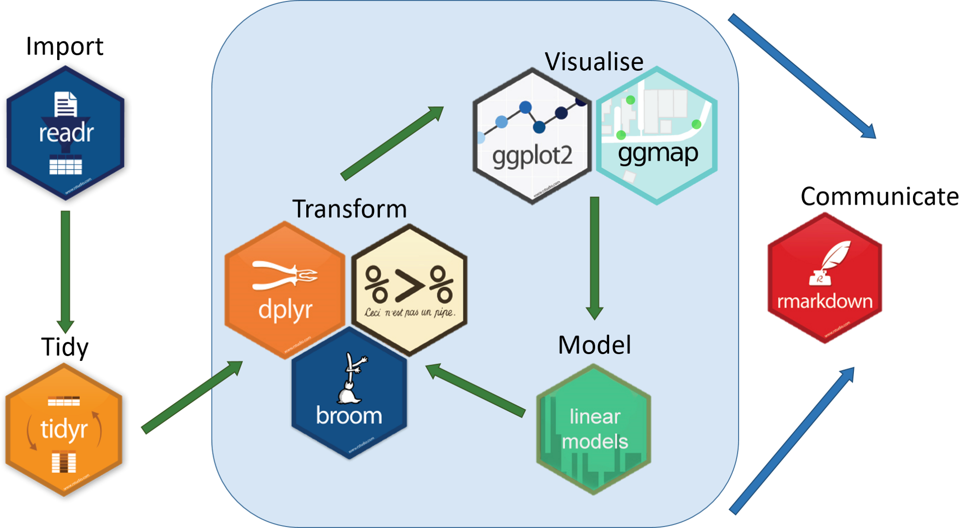] .footnote[ As a set of principles: Human-centered, Consistent, Composable, Inclusive] --- background-image: url(./images/magrittr.png) background-position: 95% 5% background-size: 10% ### The Pipe operator **%>%** _(and then)_ .center[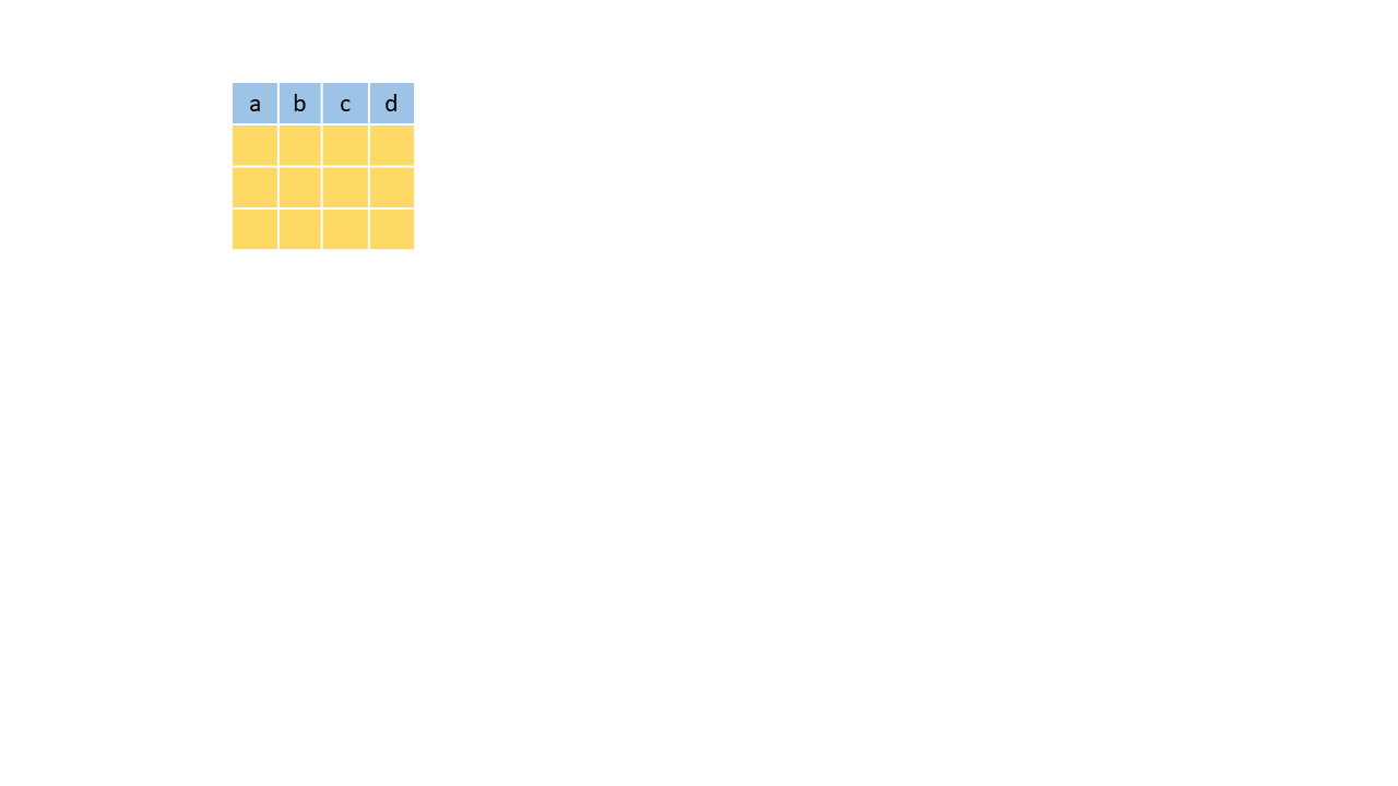] --- background-image: url(./images/magrittr.png) background-position: 95% 5% background-size: 10% ### The Pipe operator **%>%** _(and then)_ .center[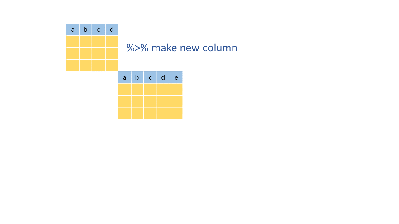] .footnote[**Shortcut:** Control/Cmd + shift + m] --- background-image: url(./images/magrittr.png) background-position: 95% 5% background-size: 10% ### The Pipe operator **%>%** _(and then)_ .center[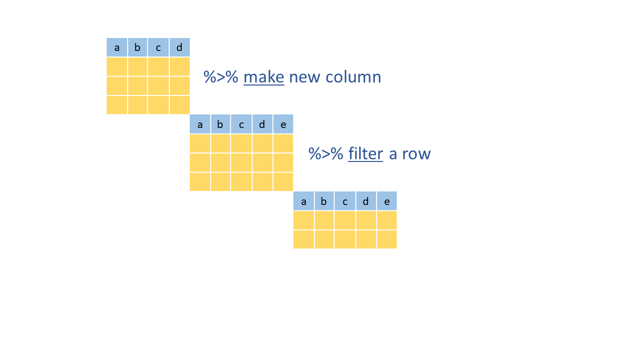] .footnote[**Shortcut:** Control/Cmd + shift + m] --- background-image: url(./images/magrittr.png) background-position: 95% 5% background-size: 10% ### The Pipe operator **%>%** _(and then)_ .center[] .footnote[**Shortcut:** Control/Cmd + shift + m] --- #R base vs. tidyverse .left[ ####Base R: **starwars**[**starwars**$height <200& **starwars**$gender == "male",] ] -- <br><br> .pull-right[ ####Tidyverse: **starwars** %>% filter(height <200, gender == "male") ] --- # R base vs. tidyverse .left[ #### Base R: **starwars**$bmi <- **starwars**$mass/(**starwars**$height/100)^2) ] -- <br><br> .pull-right[ #### Tidyverse: **starwars** %>% mutate(bmi = mass/((height/100)^2)) ] --- # Hands on! Best option: - Sign to Rstudio cloud, and join the [**project**](https://bit.ly/2Bvq6ap). - Make a **permanent copy** by clicking at right top corner. Or - Download the project folder and work on your Rstudio ### In any case open: **02_R**, **workshop.Rmd** - Open the tidyverse library ```r library(tidyverse) library(here) ``` --- # The dataset We will use 2 sets of data from the TV series **Game of thrones**: 1) `got_char.csv`: the total of minutes and seconds in TV per season for each character. 2) `got_houses.csv`: gender and the house each character represents. **#nospoilers** .footnote[ 1) Source: <i class="fab fa-github "></i> [benkahle/bayesianGameofThrones](https://github.com/benkahle/bayesianGameofThrones) 2) Source: <i class="fab fa-github "></i> [Preetish/GoT_screen_time](https://github.com/Preetish/GoT_screen_time)] --- background-image: url(./images/readr.png) background-position: 95% 5% background-size: 10% # Import files Consider type of files: * We use `read_csv` for files delimited by commas * Use `read_csv2` for files delimited by semicolon -- * If you use data in SPSS, Stata, SAS, the best package is [rio](https://cran.r-project.org/web/packages/rio/vignettes/rio.html) - It is a Swiss knife that wraps all packages - Only one function to import any kind of file: `import()` - Only one function to export any kind of file: `export()` --- background-image: url(./images/drake_nohex.jpg) background-position: 95% 5% background-size: 10% # About reproducibility <br><br><br> - **AVOID** absolute paths or setting/clearing directory using **R Projects** ```r got_char <- read_csv("C:/Users/palol/Dropbox/github/ tidyverse_workshop_oscr/01_data/got_char.csv") ``` .footnote[Check [this post](https://www.tidyverse.org/blog/2017/12/workflow-vs-script/) to understand why [Jenny Bryan](https://rstudio.com/speakers/jenny-bryan/) will come and set your computer on 🔥 if your first line in your R scripts are `setwd("C:\Users\paloma\path\that\only\I\have")` or `rm(list = ls())`] --- background-image: url(./images/drake_yeshex.jpg) background-position: 95% 5% background-size: 10% # About reproducibility - Use relative paths ```r got_char <- read_csv("../01_data/got_char.csv") ``` - Even better, use `readr` + `here` ```r got_char <- read_csv(here("01_data", "got_char.csv")) ``` .footnote[Check [this post](https://malco.io/2018/11/05/why-should-i-use-the-here-package-when-i-m-already-using-projects/) to understand why to use `here` inside projects] --- # Import with `read_csv` ```r got_char <- read_csv(here("01_data", "got_char.csv")) got_houses <- read_csv(here("01_data", "got_houses.csv")) ``` --- ### Exercise 1. Building the Top 10 within the first 3 seasons <table class="table table-hover table-condensed table-responsive" style="font-size: 16px; width: auto !important; margin-left: auto; margin-right: auto;"> <thead> <tr><th style="border-bottom:hidden; padding-bottom:0; padding-left:3px;padding-right:3px;text-align: center; " colspan="3"><div style="border-bottom: 1px solid #ddd; padding-bottom: 5px; ">TOP 10 Characters</div></th></tr> <tr> <th style="text-align:left;font-weight: bold;"> Character </th> <th style="text-align:right;font-weight: bold;"> Total acting time </th> <th style="text-align:left;font-weight: bold;"> House </th> </tr> </thead> <tbody> <tr> <td style="text-align:left;"> Tyrion Lannister </td> <td style="text-align:right;"> 167.75 </td> <td style="text-align:left;"> House Lannister </td> </tr> <tr> <td style="text-align:left;"> Jon Snow </td> <td style="text-align:right;"> 124.50 </td> <td style="text-align:left;"> Night's Watch </td> </tr> <tr> <td style="text-align:left;"> Daenerys Targaryen </td> <td style="text-align:right;"> 123.50 </td> <td style="text-align:left;"> House Targaryen </td> </tr> <tr> <td style="text-align:left;"> Arya Stark </td> <td style="text-align:right;"> 98.75 </td> <td style="text-align:left;"> House Stark </td> </tr> <tr> <td style="text-align:left;"> Eddard 'Ned' Stark </td> <td style="text-align:right;"> 92.50 </td> <td style="text-align:left;"> House Stark </td> </tr> <tr> <td style="text-align:left;"> Sansa Stark </td> <td style="text-align:right;"> 91.50 </td> <td style="text-align:left;"> House Stark </td> </tr> <tr> <td style="text-align:left;"> Cersei Lannister </td> <td style="text-align:right;"> 86.25 </td> <td style="text-align:left;"> House Lannister </td> </tr> <tr> <td style="text-align:left;"> Catelyn Stark </td> <td style="text-align:right;"> 82.75 </td> <td style="text-align:left;"> House Stark </td> </tr> <tr> <td style="text-align:left;"> Theon Greyjoy </td> <td style="text-align:right;"> 79.50 </td> <td style="text-align:left;"> House Greyjoy </td> </tr> <tr> <td style="text-align:left;"> Robb Stark </td> <td style="text-align:right;"> 77.75 </td> <td style="text-align:left;"> House Stark </td> </tr> </tbody> </table> --- background-image: url(./images/dplyr.png) background-position: 95% 5% background-size: 10% ## Dplyr package `Dplyr` is a package that provides a set of tools for efficiently manipulating datasets in R. Today we will learn the following functions: .pull-left[ - mutate - arrange - select - rename] .pull-right[ - slice - left_join (and family of joins) - group_by - summarise/summarize ] --- ## 1. Merge the two tables with `left_join` .pull-left[ 1. Pick identifier/key variables on each datase - got_char = **actor** - got_houses = **name** 2. Choose how you want to merge ] -- .pull-right[  ] .footnote[[Animated joins by @gadenbuie](https://github.com/gadenbuie/tidyexplain)] --- ## 2. Make new columns with `mutate` ```r got_complete %>% mutate(total = season_1 + season_2 + season_3) ``` .pull-left[  ] .pull-right[ - Make new variables a) With a specific value b) Based on other variables c) Change an existing variable ] .footnote[Art by [Allison Horst](https://github.com/allisonhorst)] --- ## 3. Reorganize your rows with `arrange` .pull-left[ Ascending ```r got_complete %>% arrange(total) ``` Descending ```r got_complete %>% arrange(desc(total)) ``` ] .pull-right[  ] --- ## 4. Select/remove columns with `select` ```r got_complete %>% select(actor, total, house_a) ``` -- Helpful feats of `select` a) starts_with("season") b) contains("hous") c) matches("_[:digit:]") d) -actor e) -c(actor, total) f) everything() --- ## 5. **`rename`** variables new name = old name ```r got_complete %>% rename(Character = actor, House = house_a, `Total acting time` = total) ``` ## 6. **`slice`** rows ```r got_complete %>% slice(1:10) ``` --- ## Pipe all steps and...ta da! ```r got_char %>% left_join(got_houses, by = c("actor" = "name")) %>% mutate(total = (season_1 + season_2 + season_3)) %>% arrange(desc(total)) %>% select(actor, total, house_a) %>% slice(1:10) %>% rename(Character = actor, House = house_a, `Total acting time` = total) ``` --- <br><br><br> --- ### Exercise 2. How is the gender distribution across houses? <img src="index_files/figure-html/unnamed-chunk-16-1.png" width="864" /> --- ## 1. Explore the variables with `count` .pull-left[ ```r got_houses %>% count(gender) ``` ] -- .pull-right[ ```r got_houses %>% count(house_a, sort = TRUE) %>% slice(1:4) ``` ] --- ## 2. Drop missing observations (rows) with `drop_na` ```r got_houses %>% drop_na(gender, house_a) ``` --- ## 3. Do operations within categories of a variable with `group_by` .pull-left[ ```r got_houses %>% group_by(house_a) %>% mutate(n = n()) %>% ungroup() ``` **n()** gives the current group size. ] .pull-right[  ] --- ## 4. `Filter` rows with a criteria  .footnote[Art by [Allison Horst](https://github.com/allisonhorst)] --- ## 4. Filter How would you filter houses that have at least 10 characters? a) `got_houses %>% filter(n >= 10)` b) `got_houses %>% filter(n < 10)` c) `got_houses %>% filter(houses_a >= 10)` --- ## 5. Make labels for gender ### Using `ifelse`, only 2 conditions ifelse(`condition`, **TRUE**, FALSE) ```r got_houses %>% mutate(gender = ifelse(gender == 0, "Female", "Male")) ``` Tip: Use **`case_when`** for more than two conditions --- ## Data ready to be plotted! ```r got_houses_plot <- got_houses %>% drop_na(gender, house_a) %>% group_by(house_a) %>% mutate(n = n()) %>% ungroup() %>% filter(n > 10) %>% mutate(gender = ifelse(gender == 0, "Female", "Male")) ``` -- ```r got_houses_plot %>% head(4) ``` ``` ## # A tibble: 4 x 4 ## house_a gender name n ## <chr> <chr> <chr> <int> ## 1 House Frey Male Aegon Frey (Jinglebell) 38 ## 2 House Targaryen Male Aegon Targaryen 23 ## 3 House Greyjoy Male Adrack Humble 25 ## 4 Night's Watch Male Aemon Targaryen (son of Maekar I) 104 ``` --- ## `ggplot` grammar .pull-left[ **Data** = tibble **Aesthetics** = variables to be plotted **Geometries** = Type of plot **Theme** = colors and details We go from **`%>%`** for a **`+`** for each layer ] .pull-right[  ] .footnote[[Adapted picture from @CedScherer](https://twitter.com/CedScherer/status/1229392907234402305/photo/2)] --- ## 1. Let's start with a basic bar plot .pull-left[ ```r got_houses_plot %>% ggplot(aes(house_a)) + geom_bar() ``` ] .pull-right[ <img src="index_files/figure-html/unnamed-chunk-25-1.png" width="504" /> ] --- ## 2. Now let's add add gender to aes() .pull-left[ ```r got_houses_plot %>% ggplot(aes(house_a, * fill = gender)) + geom_bar() ``` ] .pull-right[ <img src="index_files/figure-html/unnamed-chunk-27-1.png" width="504" /> ] --- ## 3. Flip the coords .pull-left[ ```r got_houses_plot %>% * ggplot(aes(y = house_a, fill= gender)) + geom_bar() ``` ] .pull-right[ <img src="index_files/figure-html/unnamed-chunk-29-1.png" width="504" /> ] Before `ggplot2 3.3.0` (last version) we needed to use `coord_flip()` --- ## 4. Sort by frequency .pull-left[ ```r got_houses_plot %>% * ggplot(aes(y = reorder(house_a, n), fill= gender)) + geom_bar() ``` ] .pull-right[ <img src="index_files/figure-html/unnamed-chunk-31-1.png" width="504" /> ] --- ## 5. Details count 💅🏽 ```r got_houses_plot %>% ggplot(aes(y = reorder(house_a, n), fill= gender)) + geom_bar() + labs(title = "Distribution of gender across the houses", x = "Number of characters", y = "House", fill = "Gender") + theme_minimal() ``` --- <br><br><br> .center[ <img src="index_files/figure-html/unnamed-chunk-33-1.png" width="864" /> ] --- ## Exercise 3. How was the evolution of the protagonists across seasons? <img src="index_files/figure-html/unnamed-chunk-34-1.png" width="1008" /> **What variables do we need to plot this graph?** --- ## What is tidy data .pull-left[ - **Rule 1**: Each **_variable_** must have its own **_column_**. <br><br><br><br><br><br> - **Rule 2**: Each **_observation_** must have its own **_row_**. <br><br><br><br><br><br> - **Rule 3**: Each **_value_** must have its own **_cell_**. ] .pull-right[ <center>  <center> ] .foot-note[https://r4ds.had.co.nz/] --- background-image: url(./images/tidyr.png) background-position: 95% 5% background-size: 8% ### Go from wide to long with `pivot_longer`  --- background-image: url(./images/tidyr.png) background-position: 95% 5% background-size: 8% ### Go from wide to long with `pivot_longer` ```r got_complete %>% pivot_longer( cols = season_1:season_7, names_to = "season", values_to = "time", names_prefix = "season_") head(got_long) ``` --- background-image: url(./images/tidyr.png) background-position: 95% 5% background-size: 8% ### Go from wide to long with `pivot_longer` ```r got_complete %>% pivot_longer( * cols = season_1:season_7, names_to = "season", values_to = "time", names_prefix = "season_") ```  --- background-image: url(./images/tidyr.png) background-position: 95% 5% background-size: 8% ### Go from wide to long with `pivot_longer` ```r got_complete %>% pivot_longer( cols = season_1:season_7, * names_to = "season", values_to = "time", names_prefix = "season_") ```  --- background-image: url(./images/tidyr.png) background-position: 95% 5% background-size: 8% ### Go from wide to long with `pivot_longer` ```r got_complete %>% pivot_longer( cols = season_1:season_7, names_to = "season", * values_to = "time", names_prefix = "season_") ```  --- background-image: url(./images/tidyr.png) background-position: 95% 5% background-size: 8% ### Go from wide to long with `pivot_longer` ```r got_long <- got_complete %>% pivot_longer( cols = season_1:season_7, names_to = "season", values_to = "time", * names_prefix = "season_") ``` --- ### Create a total sum of time by character .pull-left[ **`group_by() + summarise()`** ```r got_long %>% group_by(actor) %>% summarise (total = sum(time)) %>% ungroup () ```  ] -- .pull-left[ **`group_by() + mutate()`** ```r got_long %>% group_by(actor) %>% mutate(total = sum(time)) %>% ungroup() ```  ] --- ### Back to the graph <img src="index_files/figure-html/unnamed-chunk-44-1.png" width="864" /> --- ### 1. Add the aesthetics and geoms .pull-left[ ```r got_long %>% ggplot(aes(season, time))+ geom_point() + geom_line() ``` ] .pull-right[ <img src="index_files/figure-html/unnamed-chunk-46-1.png" width="504" /> ] --- ### 2. Add actors to aes() .pull-left[ ```r got_long %>% ggplot(aes(season, time, * group = actor)) + geom_point() + geom_line() ``` ] .pull-right[ <img src="index_files/figure-html/unnamed-chunk-48-1.png" width="504" /> ] --- ### 3. Filter the top ten (>130min) .pull-left[ ```r got_long %>% filter(total >130) %>% ggplot(aes(season, time, group = actor))+ geom_point() + geom_line() ``` ] .pull-right[ <img src="index_files/figure-html/unnamed-chunk-50-1.png" width="504" /> ] --- ### 4. Add a color for each character .pull-left[ ```r got_long %>% filter(total >130) %>% ggplot(aes(season, time, group = actor, * color = actor)) + geom_point() + geom_line() ``` ] .pull-right[ <img src="index_files/figure-html/unnamed-chunk-52-1.png" width="504" /> ] --- ### 5. Details ```r got_long %>% filter(total >130) %>% ggplot(aes(season, time, group = actor, color = actor)) + geom_point() + geom_line() + theme_minimal() + labs(title = "Evolution of the protagonists across seasons", x = "Season", y = "Total time (min)", color = "Protagonist") + theme_minimal() ``` --- ### Final graph <img src="index_files/figure-html/unnamed-chunk-54-1.png" width="864" /> --- background-image: url("https://gph.to/2GrDSdk") background-position: 50% 50% # We did it! --- # Useful resources - Learn tidyverse with the R4DS book (free online): https://r4ds.had.co.nz/ - Practice your skills with the primers: https://rstudio.cloud/learn/primers - Join the R4DS and Tidy-tuesday community in twitter --- name: title class: center, middle #Thank you!!!# ###Keep in touch! <i class="fas fa-paper-plane " style="color:#011A5E;"></i></i> l.rojassaunero@erasmusmc.nl</a><br> <i class="fab fa-twitter " style="color:#011A5E;"></i> <a href="http://twitter.com/palolili23"> </i> @palolili23</a><br> <i class="fab fa-github " style="color:#011A5E;"></i> <a href="http://twitter.com/palolili23"> </i> @palolili23</a><br>