pubmed_webscrap
Gender proportions in NEJM
The following analysis was inspired by the work of Megan Frederickson, “Covid-19’s gendered impact on academia productivity” available here.
Data was collected from all publications registered in pubmed, from the New England Journal of Medicine, from 1945 to 2020. (Raw data available at 01_data)
Since all publications only had first name initials, I used the package
rcrossref, function cr_cn,
which gets citation in various formats from CrossRef and only requires
the DOI. Before pulling the citations, I registered for the Polite
Pool
as good practices, and requires setting my email account in the
Renviron. I used the cr_cn with the default setting, which pulls
article data in bibtex format,
which has complete names for all authors. The code for this step can be
found in
02_r/extract_bib.
I did it in batches of ~10000 and saved the new dataframes with the
bibtex data as .Rda, they can be found at
01b_clean_data/nejm.
Once all papers had their bibtex information, I followed the next steps to clean the data:
library(tidyverse)
Steps to import the data:
data_dir <- "01b_clean_data/nejm"

rda_files <- fs::dir_ls(data_dir, regexp = "\\.Rda$")

data <- rda_files %>%
  map_dfr(rio::import)

data <- data %>%
  distinct(PMID, .keep_all = TRUE)

data %>%
  select(DOI, bib) %>%
  sample_n(3) %>%
  mytable()
| DOI | bib |
|---|---|
| 10.1056/nejm197811162992019 | @article{1978, doi = {10.1056/nejm197811162992019}, url = {<https://doi.org/10.1056%2Fnejm197811162992019>}, year = 1978, month = {nov}, publisher = {Massachusetts Medical Society}, volume = {299}, number = {20}, pages = {1137–1137}, title = {Blood Pressure in Coffee Drinkers}, journal = {New England Journal of Medicine} } |
| 10.1056/NEJMc080368 | @article{2008, doi = {10.1056/nejmc080368}, url = {<https://doi.org/10.1056%2Fnejmc080368>}, year = 2008, month = {jun}, publisher = {Massachusetts Medical Society}, volume = {358}, number = {24}, pages = {2641–2644}, title = {Drug-Eluting Stents vs. Coronary-Artery Bypass Grafting}, journal = {New England Journal of Medicine} } |
| 10.1056/NEJM199603283341316 | @article{Melero\_Pita\_1996, doi = {10.1056/nejm199603283341316}, url = {<https://doi.org/10.1056%2Fnejm199603283341316>}, year = 1996, month = {mar}, publisher = {Massachusetts Medical Society}, volume = {334}, number = {13}, pages = {866–867}, author = {A. Melero-Pita and F. Alonso-Pardo and J.L. Bardaj{'{}}-Mayor and J. Higueras}, title = {Corrected Transposition of the Great Arteries}, journal = {New England Journal of Medicine} } |
Extract authors name and make as many rows as authors, per paper
# Create an author variable from the bibtex
data <- data %>% mutate(
  author = str_extract(bib, "(author = \\{)(.)+"),
  author = str_remove(author, "author = \\{"),
  author = str_remove(author, "\\},")
)

## Separate authors into multiple columns using the split_into_multiple function.
## Create as many rows as authors for each paper using pivot_longer

split_into_multiple <- function(column, pattern = ", ", into_prefix){
  cols <- str_split_fixed(column, pattern, n = Inf)
  cols[which(cols == "")] <- NA
  cols <- as_tibble(cols)
  m <- dim(cols)[2]

  names(cols) <- paste(into_prefix, 1:m, sep = "_")
  return(cols)
}

data_authors <- data %>%
  bind_cols(split_into_multiple(data$author, " and ", "author")) %>%
  pivot_longer(
    cols = starts_with("author_"),
    names_to = "author_position",
    values_to = "author_name",
    names_prefix = "author_") %>%
  drop_na(author_name)


# Some authors only have initials instead of complete first names, these will be excluded
# Separate first and last name

data_authors <- data_authors %>%
  mutate(author_clean = str_remove_all(author_name, "[:upper:][:punct:]"),
         author_clean = str_trim(author_clean, side = "both")) %>%
  separate(author_clean, into = c("first_name", "last_name"), fill = "left")

data_filtered <- data_authors %>%
  drop_na(first_name)

data_filtered %>%
filter(DOI == "10.1056/nejm194511152332004") %>%
  select(author_position, author_name, first_name, last_name) %>%
  mytable()
| author\_position | author\_name | first\_name | last\_name |
|---|---|---|---|
| 1 | Elliot L. Sagall | Elliot | Sagall |
| 2 | Albert Dorfman | Albert | Dorfman |
Find gender for each author
To identify the gender of each author, I use the gender
package, by Mullen, L. (2019).
gender: Predict Gender from Names Using Historical Data. R package
version 0.5.3 and the U.S. Social Security Administration baby names
database. To use the gender function, the package asks to download the
genderdata package, but installation can be tricky as discussed in
this post. I downloaded the package
using devtools::install_github("ropensci/genderdata") command.
Considerations: This package attempts to infer gender (or more precisely, sex assigned at birth) based on first names using historical data. This method has many limitations as discussed here, which include its reliance of data created by the state and its inability to see beyond the state-imposed gender binary and is meant to be used for studying populations in the aggregate. This method is a rough approach and can missclassify gender or exclude individual authors, but it can give a picture of the gender bias within the large dataset.
names <- data_filtered %>% count(first_name) %>% pull(first_name)

gender <- gender::gender(names, method = "ssa")

data_filtered <- data_filtered %>%
  left_join(gender, by = c("first_name" = "name")) %>%
  select(-starts_with("proportion"),
         -starts_with("year"))

data_filtered %>%
  select(first_name, gender) %>%
  group_by(gender) %>%
  sample_n(2) %>%
  mytable()
| first\_name | gender |
|---|---|
| Aubrey | female |
| Betty | female |
| Fergus | male |
| Philip | male |
| Gatana | NA |
| Bhabita | NA |
Plot
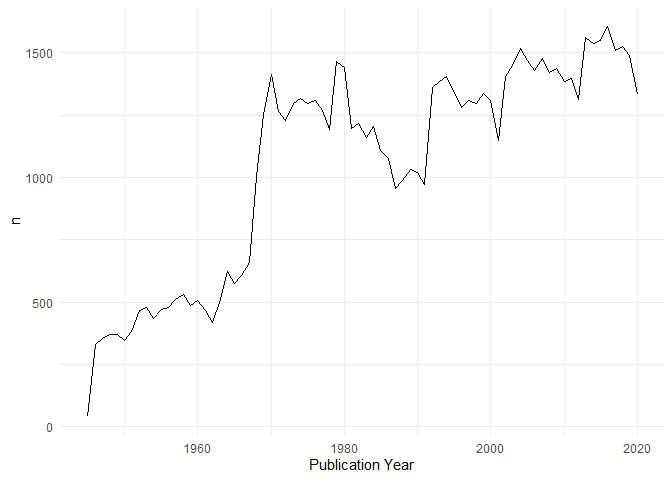
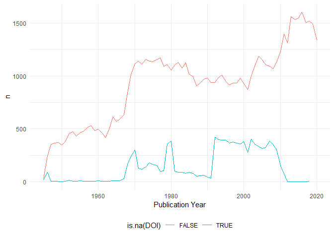
Insight on the number of papers per year, and number of missing papers with missing DOI
For the following plots I will make slight changes to the gender variable:
data_filtered <- data_filtered %>%
  mutate(
    `Publication Year` = as_factor(`Publication Year`),
    gender = ifelse(is.na(gender), "unknown", gender),
    gender = ifelse(is.na(gender), "unknown", gender),
    gender = str_to_title(gender)) %>%
  group_by(DOI) %>%
  mutate(total_authors = last(author_position)) %>%
  ungroup() %>%
  mutate(gender = fct_relevel(gender, c("Unknown", "Male", "Female")))
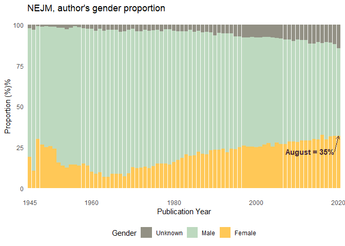
Gender proportion over time
count_gender <- data_filtered %>%
  group_by(`Publication Year`) %>%
  count(gender) %>%
  mutate(prop = round(100*n/sum(n), 2)) %>%
  ungroup()

count_gender %>%
  ggplot(aes(`Publication Year`, prop, fill = gender)) +
  geom_col() +
  scale_fill_manual(values = c("#929084", "#BDD9BF", "#FFC857")) +
  theme_minimal() +
  labs(title = "NEJM, author's gender proportion",
     y = "Proportion (%)%",
     fill = "Gender") +
  scale_x_discrete(breaks = c("1945", "1960", "1980", "2000", "2020")) +
    theme(legend.position = "bottom")+
  theme(panel.grid = element_blank()) +
   annotate(
    geom = "curve", x = 75, y = 22, xend = 76, yend = 32,
    curvature = 0.0, arrow = arrow(length = unit(2, "mm")), color = "#412234", size = 0.7) +
  annotate(geom = "text", x = 75, y = 22.5, label = "August = 35%", hjust = "right", color = "#412234", size = 4,
           fontface="bold")
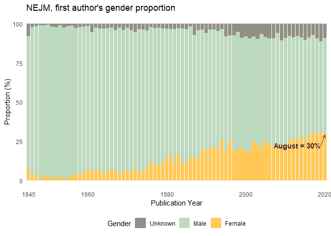
First author´s gender proportion over time
count_gender_first <- data_filtered %>%
  filter(author_position == 1,
         total_authors != 1) %>%
  group_by(`Publication Year`) %>%
  count(gender) %>%
  mutate(prop = round(100*n/sum(n), 2)) %>%
  ungroup()

count_gender_first %>%
  ggplot(aes(`Publication Year`, prop, fill = gender)) +
  geom_col() +
  scale_fill_manual(values = c("#929084", "#BDD9BF", "#FFC857")) +
  theme_minimal() +
  labs(
    title = "NEJM, first author's gender proportion",
    y = "Proportion (%)",
    fill = "Gender") +
    scale_x_discrete(
    breaks=c("1945", "1960", "1980", "2000", "2020")) +
    theme(legend.position = "bottom",
          panel.grid = element_blank()) +
 annotate(
    geom = "curve", x = 75, y = 22, xend = 76, yend = 29,
    curvature = 0.0, arrow = arrow(length = unit(2, "mm")), color = "#412234", size = 0.7) +
  annotate(geom = "text", x = 75, y = 22.5, label = "August = 30%", hjust = "right", color = "#412234", size = 4,
           fontface="bold")
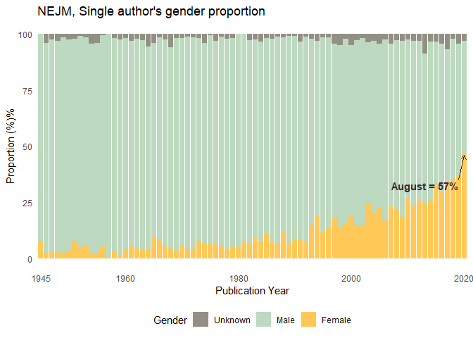
Single author´s proportion over time
count_single <- data_filtered %>%
  filter(total_authors == 1) %>%
  group_by(`Publication Year`) %>%
  count(gender) %>%
  mutate(prop = round(100*n/sum(n), 2)) %>%
  ungroup()

count_single %>%
  ggplot(aes(`Publication Year`, prop, fill = gender)) +
  geom_col() +
  scale_fill_manual(values = c("#929084", "#BDD9BF", "#FFC857")) +
  theme_minimal() +
  labs(
    title = "NEJM, Single author's gender proportion",
    y = "Proportion (%)%",
    fill = "Gender") +
    scale_x_discrete(
    breaks=c("1945", "1960", "1980", "2000", "2020")
  ) +
    theme(legend.position = "bottom",
          panel.grid = element_blank()) +
   annotate(
    geom = "curve", x = 75, y = 35, xend = 76, yend = 46,
    curvature = 0.0, arrow = arrow(length = unit(2, "mm")), color = "#412234", size = 0.7) +
  annotate(geom = "text", x = 75, y = 32.5, label = "August = 57%", hjust = "right", color = "#412234", size = 4,
           fontface="bold")
Last author’s gender proportion
count_last<- data_filtered %>%
  filter(total_authors != 1,
         author_position == total_authors) %>%
  group_by(`Publication Year`) %>%
  count(gender) %>%
  mutate(prop = round(100*n/sum(n), 2)) %>%
  ungroup()

count_last %>%
  ggplot(aes(`Publication Year`, prop, fill = gender)) +
  geom_col() +
  scale_fill_manual(values = c("#929084", "#BDD9BF", "#FFC857")) +
  theme_minimal() +
  labs(
    title = "NEJM, Last author's gender proportion",
    y = "Proportion (%)%",
    fill = "Gender") +
    scale_x_discrete(
    breaks=c("1945", "1960", "1980", "2000", "2020")
  ) +
    theme(legend.position = "bottom",
          panel.grid = element_blank())+
   annotate(
    geom = "curve", x = 75, y = 17, xend = 76, yend = 24.5,
    curvature = 0.0, arrow = arrow(length = unit(2, "mm")), color = "#412234", size = 0.7) +
  annotate(geom = "text", x = 75, y = 17.5, label = "August = 34%", hjust = "right", color = "#412234", size = 4,
           fontface="bold")
